Modeling Expected Points with the Poisson Distribution

Expected points (xP) in soccer as an analytics concept is fairly new, but it is growing in popularity in recent times, as of April 2023. The idea behind it and how it is calculated is less well-known, so I’d like to take the chance with this post to dive deeper into expected points, with an illustrative toy example that poses the idea in an interesting way. A post from Tony’s Blog was the inspiration for this post as well, so I wanted to give a shout out.

The expected points concept is predicated on the expected goals (xG) model. Expected goals has also gained recent traction naturally as well, and it’s important to understand expected goals first. Said in few words, the expected goals model quantifies the idea that “not all shots taken are equal.” The model produces a probability of a goal being scored, for any particular shot. It’s very interesting, and if you are wanting to learn more, check out this link. But at the end of the day, again, the important takeaway is that the model produces a probability that a goal will be scored from a given shot.

Let’s start with the example that I will walk through in this post. Say you have two teams playing in a match, Team A and Team B. In the 90 minutes, Team A took eight shots, and each shot had an probability (xG) of 0.1. Then, Team B took three shots, and the shots had probabilities of 0.2, 0.3, and 0.3. Now in this example, each team has a total xG of 0.8. Let’s pause and start expressing this as code.

First, I will import all the necessary libraries. Then, I will store the probabilities for each team’s shots in a NumPy array and calculate the xG for each team.

import numpy as np
import pandas as pd
import matplotlib.pyplot as plt
import seaborn as sns
from poibin import PoiBin

xg_A = np.array([.1] * 8)
xg_B = np.array([.2, .3, .3])

print(f"Goal probabilities for {len(xg_A)} shots by Team A: {xg_A.tolist()}")
print(f"Goal probabilities for {len(xg_B)} shots by Team B: {xg_B.tolist()}\n")
print(f"Total xG for Team A: {xg_A.sum()}")
print(f"Total xG for Team B: {xg_B.sum()}")

Goal probabilities for 8 shots by Team A: [0.1, 0.1, 0.1, 0.1, 0.1, 0.1, 0.1, 0.1]
Goal probabilities for 3 shots by Team B: [0.2, 0.3, 0.3]

Total xG for Team A: 0.8
Total xG for Team B: 0.8

As you can see, each team has an identical total xG (simply the sum of the probabilities of the shots taken) for the game, even though Team A has eight shots to Team B’s three. The question I’d like to pose is this:

Even though the total xG is identical, is it better to have more shots with lower probabilities or fewer shots with higher probabilities, in terms of the probability of victory and expected points (xP)?

To answer this question, let’s use the Poisson distribution, and eventually expected points for the analysis. The Poisson distribution is a foundational discrete statistical distribution, and it expresses the probability of a number of events occurring in a fixed time interval. If you want to learn more, you can check out this great article.

It’s important to note that the Poisson model has some assumptions that we are relaxing here in this case. For example, the model assumes that events are independent. You can make a very good argument that goals scored in a game are not independent; a good example might be that a team that concedes a goal may play more aggressively when chasing the game, leaving them open to conceding another goal. I’m curious to hear thoughts on this! But in any case, let’s relax these and follow through.

Typically, when you work with the Poisson distribution, you find the maximum likelihood estimate for lambda, which is the average number of events (goals) in the fixed time interval (90 minutes for a match). In our case, we don’t have that; we only have the goal probabilities. Luckily, methods to construct the Poisson distribution functions that we need have been developed, and you can read more about that in this paper. In fact, the poibin library that I imported is based on that paper, and you can find the github for that library here. But at the end of the day, all you have to know is that we are constructing the Poisson distributions by passing the goal probabilities of the shots for each team.

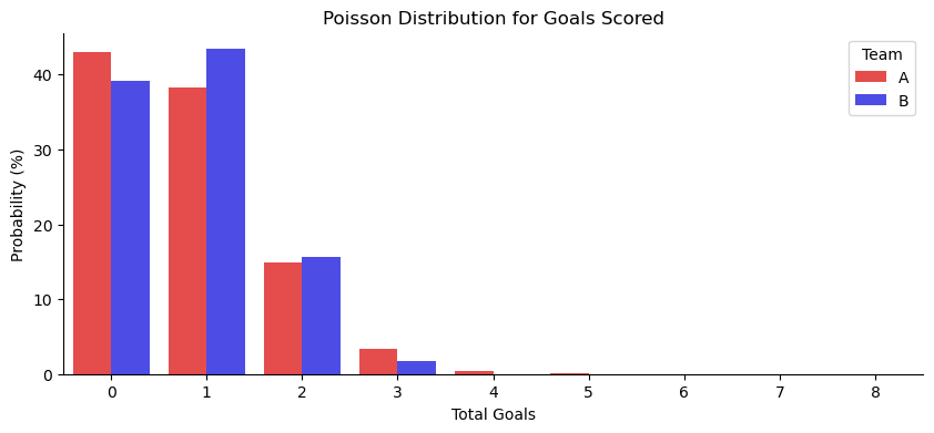
Now we can continue expressing this idea in code. First, I construct the Poisson distributions for both teams by passing the shot probabilities. Then, I use the probability mass functions from each distribution to get the probabilities that the teams score a particular number of goals, up to the amount of shots taken (eight in this case). I printed out the two vectors so you can see what they look like. Additionally, I’ll show a simple visualization for the Poisson distributions.

pd_A = PoiBin(xg_A)
pd_B = PoiBin(xg_B)

total_goal_prob_A = np.array([pd_A.pmf(i) for i in range(len(xg_A)+1)])
total_goal_prob_B = np.array([pd_B.pmf(i) for i in range(len(xg_B)+1)] + [0] * (len(xg_A) - len(xg_B)))


print(f"Probability of total goals scored for Team A:\n{[(goal, round(prob,4)) for goal, prob in enumerate(total_goal_prob_A)]}")
print("\n")
print(f"Probability of total goals scored for Team B:\n{[(goal, round(prob,2)) for goal, prob in enumerate(total_goal_prob_B)]}\n\n")

goal_probs = pd.DataFrame({"Goals": range(len(total_goal_prob_A)),
                          "A": total_goal_prob_A * 100,
                          "B": total_goal_prob_B * 100}).melt(id_vars=["Goals"], var_name="Team", value_name="Probability")

fig, axs = plt.subplots(1,1, figsize = (10,4))
sns.barplot(data = goal_probs, x = "Goals", y = "Probability", hue = "Team", palette = ['r', 'b'], alpha = 0.8)
sns.despine()

_=plt.title("Poisson Distribution for Goals Scored")
_=plt.ylabel("Probability (%)")
_=plt.xlabel("Total Goals")

Probability of total goals scored for Team A:
[(0, 0.4305), (1, 0.3826), (2, 0.1488), (3, 0.0331), (4, 0.0046), (5, 0.0004), (6, 0.0), (7, 0.0), (8, 0.0)]


Probability of total goals scored for Team B:
[(0, 0.39), (1, 0.43), (2, 0.16), (3, 0.02), (4, 0.0), (5, 0.0), (6, 0.0), (7, 0.0), (8, 0.0)]

With those steps complete, I can construct a table of joint probabilities that summarizes the various possible match outcomes probabilistically, which will be very useful for our analysis. I did this by taking the outer product of the two probability vectors of total goals scored for the teams. You can think of this table as showing the probability of all the possible match outcomes.

match_probs = pd.DataFrame(np.outer(total_goal_prob_A, total_goal_prob_B), 
             index = [str(i) + " goals for A" for i in range(len(total_goal_prob_A))], 
             columns = [str(i) + " goals for B" for i in range(len(total_goal_prob_B))])

match_probs.round(5)

	0 goals for B	1 goals for B	2 goals for B	3 goals for B	4 goals for B	5 goals for B	6 goals for B	7 goals for B	8 goals for B
0 goals for A	0.16874	0.18682	0.06715	0.00775	0.0	0.0	0.0	0.0	0.0
1 goals for A	0.14999	0.16606	0.05969	0.00689	0.0	0.0	0.0	0.0	0.0
2 goals for A	0.05833	0.06458	0.02321	0.00268	0.0	0.0	0.0	0.0	0.0
3 goals for A	0.01296	0.01435	0.00516	0.00060	0.0	0.0	0.0	0.0	0.0
4 goals for A	0.00180	0.00199	0.00072	0.00008	0.0	0.0	0.0	0.0	0.0
5 goals for A	0.00016	0.00018	0.00006	0.00001	0.0	0.0	0.0	0.0	0.0
6 goals for A	0.00001	0.00001	0.00000	0.00000	0.0	0.0	0.0	0.0	0.0
7 goals for A	0.00000	0.00000	0.00000	0.00000	0.0	0.0	0.0	0.0	0.0
8 goals for A	0.00000	0.00000	0.00000	0.00000	0.0	0.0	0.0	0.0	0.0

Next, let’s determine the probabilities for a draw, a Team A win, and a Team B win. Because I have that table of joint probabilities, we can simply sum the entries in the table that correspond to the three outcomes we care about.

I print out the results of this operation, and you can see that Team B actually has a slightly greater chance of winning! Very interesting, isn’t it? So this tells you, according to the Poisson distribution built from the shot probabilities, Team B is actually better off in terms of the probability of winning.

P_draw = np.diag(match_probs).sum()
P_A = np.tril(match_probs,-1).sum()
P_B = np.triu(match_probs,1).sum()

print(f"Probability of a draw: {P_draw.round(2)}")
print(f"Probability of a Team A victory: {P_A.round(2)}")
print(f"Probability of a Team B victory: {P_B.round(2)}")

Probability of a draw: 0.42
Probability of a Team A victory: 0.28
Probability of a Team B victory: 0.3

With these probabilities, getting the expected points for each team is trivial. All I need to do is to multiply three by the probability of winning for that team plus one times the probability of a draw (because you get three points for a win and one for a draw).

xP_A = 3 * P_A + 1 * P_draw
xP_B = 3 * P_B + 1 * P_draw

print(f"xP for Team A: {round(xP_A, 2)}")
print(f"xP for Team B: {round(xP_B, 2)}")

xP for Team A: 1.27
xP for Team B: 1.31

And that pretty much sums up the analysis! Let me know if you have any thoughts, questions, or suggestions. Thank you for taking the time to read through, and I hope you found it interesting and useful.