
Comparing Probability Distributions with Kullback-Leibler (KL) Divergence
Probability distributions are ubiquitous in data science, and you will come across and use them in some form or fashion in almost everything you do in terms of data science. An interesting operation that you can do with distributions is to quantify how different or how much “information is lost” between two distributions. One way to do this and what this post will explore is Kullback-Leibler (KL) Divergence.
One modern example of an application of KL Divergence is inside the loss function for Variational Autoencoders (VAEs). VAEs are a type of generative deep learning model, and KL Divergence is used to assist the model in creating distributions that are close to a standard normal distribution. VAEs won’t be covered in this post directly, but they are certainly a fascinating topic that I would highly recommend as future reading.
To begin exploring KL Divergence, let’s set up a toy dataset that is intuitive enough to allow you see the big picture. First, let’s import some necessary libraries.
import numpy as np
import pandas as pd
from scipy.stats import binom
import matplotlib.pyplot as plt
import seaborn as sns
With the libraries imported, I’ll create a simple dataset. The dataset is synthetic and is meant to simply store a count of goals scored by some imaginary set of players. Each of the other columns stores the probabilities of the associated goals value, and we have three different distributions represented: Observed, uniform, and binomial.
# create dataset with some toy data
samples = pd.DataFrame({"goals":[2]*3 + [3]*3 + [4]*5 + [5]*6 + [6]*3 + [7]*2 + [8]*3})
# calculate probabilities associated with each observed value
emp_probs = (samples.groupby("goals").goals.count() / len(samples)).rename("emp_probs").reset_index()
samples = samples.merge(emp_probs, on = ["goals"])
# calculate values under a uniform distribution for each observed value
samples['uniform_probs'] = 1 / samples.goals.nunique()
# calculate values under a binomial distribution constructed from observed data
samples['binomial_probs'] = samples.goals.apply(lambda x: binom.pmf(x, n = len(samples), p = samples.goals.mean()/len(samples)))
samples
| goals | emp_probs | uniform_probs | binomial_probs | |
|---|---|---|---|---|
| 0 | 2 | 0.12 | 0.142857 | 0.079725 |
| 1 | 2 | 0.12 | 0.142857 | 0.079725 |
| 2 | 2 | 0.12 | 0.142857 | 0.079725 |
| 3 | 3 | 0.12 | 0.142857 | 0.146742 |
| 4 | 3 | 0.12 | 0.142857 | 0.146742 |
| 5 | 3 | 0.12 | 0.142857 | 0.146742 |
| 6 | 4 | 0.20 | 0.142857 | 0.193764 |
| 7 | 4 | 0.20 | 0.142857 | 0.193764 |
| 8 | 4 | 0.20 | 0.142857 | 0.193764 |
| 9 | 4 | 0.20 | 0.142857 | 0.193764 |
| 10 | 4 | 0.20 | 0.142857 | 0.193764 |
| 11 | 5 | 0.24 | 0.142857 | 0.195379 |
| 12 | 5 | 0.24 | 0.142857 | 0.195379 |
| 13 | 5 | 0.24 | 0.142857 | 0.195379 |
| 14 | 5 | 0.24 | 0.142857 | 0.195379 |
| 15 | 5 | 0.24 | 0.142857 | 0.195379 |
| 16 | 5 | 0.24 | 0.142857 | 0.195379 |
| 17 | 6 | 0.12 | 0.142857 | 0.156355 |
| 18 | 6 | 0.12 | 0.142857 | 0.156355 |
| 19 | 6 | 0.12 | 0.142857 | 0.156355 |
| 20 | 7 | 0.08 | 0.142857 | 0.101888 |
| 21 | 7 | 0.08 | 0.142857 | 0.101888 |
| 22 | 8 | 0.12 | 0.142857 | 0.055037 |
| 23 | 8 | 0.12 | 0.142857 | 0.055037 |
| 24 | 8 | 0.12 | 0.142857 | 0.055037 |
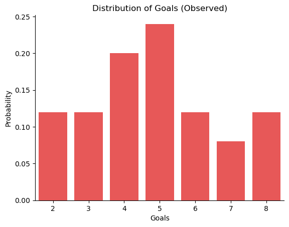
First, let’s inspect the “observed” data. The visualization below displays the distribution of the goals data.
sns.barplot(x = samples.goals,
            y = samples.emp_probs,
            color = "red",
            alpha = 0.75)

plt.title("Distribution of Goals (Observed)")
_ = plt.xlabel("Goals")
_ = plt.ylabel("Probability")
sns.despine()
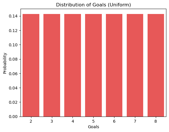
Next, let’s look at a uniform constructed to represent the goals data. In this uniform distribution, all seven unique values have the same probability, 1/7.
sns.barplot(x = samples.drop_duplicates().goals,
            y = samples.drop_duplicates().uniform_probs,
            color = "red",
            alpha = 0.75)
_ = plt.title("Distribution of Goals (Uniform)")
_ = plt.xlabel("Goals")
_ = plt.ylabel("Probability")
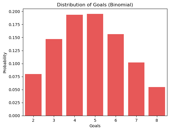
Finally, we have constructed a binomial distribution. If you are familiar with the normal distribution, you will see that it looks very similar. You can consider the binomial distribution the “normal” distribution for discrete data. The binomial distribution can be represented by two values, n and p, where n is the number of trials and p is the probability. We can estimate the probability by taking the mean of the data divided by the number of trials.
sns.barplot(x = samples.drop_duplicates().goals,
            y = samples.drop_duplicates().binomial_probs,
            color = "red",
            alpha = 0.75)
_ = plt.title("Distribution of Goals (Binomial)")
_ = plt.xlabel("Goals")
_ = plt.ylabel("Probability")
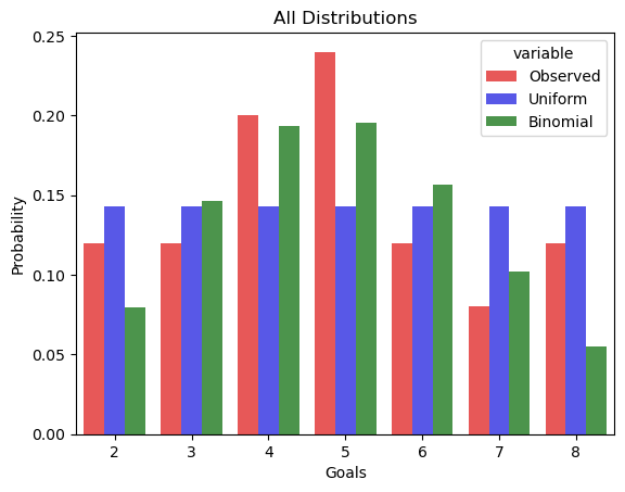
Now, let’s take a look at all distributions together.
grouped_samples = samples.melt(id_vars=["goals"]).drop_duplicates().replace({"emp_probs":"Observed", "uniform_probs":"Uniform", "binomial_probs":"Binomial"})
sns.barplot(data = grouped_samples,
            x = "goals",
            y = "value",
            hue = "variable",
            alpha = 0.75,
            palette = ["red", "blue", "green"])

plt.title("All Distributions")
plt.xlabel("Goals")
plt.ylabel("Probability")
Text(0, 0.5, 'Probability')
Now that we have our three different distributions for the data, let’s get into the implementation of KL Divergence. Below is the equation for KL Divergence, where p is the probability of the sample and q is the probability of the sample from the approximating distribution.
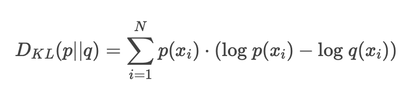
After taking this equation and implementing it in code, we can calculate the KL Divergence between the observed distribution and the uniform and binomial distributions.
def kl_divergence(p, q):
    return np.sum(p * (np.log2(p) - np.log2(q)))
print(f"KL Divergence between Observed and Uniform Distribution: {kl_divergence(samples.emp_probs, samples.uniform_probs)}")
KL Divergence between Observed and Uniform Distribution: 1.067154975387125
print(f"KL Divergence between Observed and Binomial Distribution: {kl_divergence(samples.emp_probs, samples.binomial_probs)}")
KL Divergence between Observed and Binomial Distribution: 0.792492668625009
As you can see from the results, you can see that the binomial distribution has a lower KL Divergence from the observed distribution than the uniform, so it’s a better approximation. Finally, let’s check our function to make sure it’s working how we expect. If you calculate the KL Divergence of the distribution from itself, you should get a value of 0.
print("KL Divergence Check - all results should display 0:\n"
      f"Observed - Observed: {kl_divergence(samples.emp_probs, samples.emp_probs)}\n"
      f"Uniform - Uniform: {kl_divergence(samples.uniform_probs, samples.uniform_probs)}\n"
      f"Binomial - Binomial: {kl_divergence(samples.binomial_probs, samples.binomial_probs)}\n")
KL Divergence Check - all results should display 0:
Observed - Observed: 0.0
Uniform - Uniform: 0.0
Binomial - Binomial: 0.0
And it looks like it is working well! Thank you for following this post, and I hope you found it informative.