Linear Regression from Scratch
In the past few weeks of my Applied Machine Learning course, we’ve been focusing on linear regression and its extensions. I wanted to continue my exploration of the algorithms by trying to build an implementation from scratch. A main part of this section of the course focused on gradient descent, so this implementation uses gradient descent as the main driver of the algorithm, as opposed to the closed-form solution to linear regression. As I did with K Nearest Neighbors, I built an object-oriented implementation modeled after the SKLearn “fit-predict” paradigm. Here are a few other notes about this project:
-
I am using full gradient descent here. I tried to implement a stochastic version but I was having trouble with the indexing/slicing inside the _gd function. Any tips would be very helpful!
-
The objective function that I used in this is mean squared error. Throughout this section of the course, we became familiar with the gradient of this objective function.
-
I added L2 regularization, which is also known as ridge regression. By setting the “l2_reg” hyperparameter to 0, you can “turn it off”.
-
The learning rate (eta) and regularization hyperparameter are passed at the initial instantiation of the class, opposed to at the “fit” method. Are there pros/cons to each?
-
I didn’t realize exactly how important scaling the data is for this to work. I spent a lot of time trying to figure out why gradient descent wasn’t working. Actually gradient descent was going in the opposite direction! I’ll do a little demonstration at the end to show this. It was a hard lesson to learn, but very valuable at the end of the day.
First, I will import numpy, pandas, matplotlib, and seaborn. Numpy is the foundation for this project, and I’ve used pandas to build a nicer-looking dataframe that holds the history of gradient descent. Matplotlib and seaborn are imported so that I could show some visualizations.
import numpy as np
import pandas as pd
import matplotlib.pyplot as plt
import seaborn as sns
sns.set_style('darkgrid')
Now that I have the necessary packages, I can go ahead and create the class.
class AndyLinRegGD(object):

    def __init__(self, eta = 0.001, l2_reg = 0.0):
        self.coef_ = None       # weight vector
        self.bias_ = None       # bias term
        self._theta = None      # augmented weight vector, i.e., bias + weights
        self._eta = eta         # step size for gradient descent
        self.l2_reg = l2_reg    # control parameter for regularization penalty term

        #gradient descent history, will build as DataFrame in later function
        self.history = {"MSE": [],
                       "Updated Weights":[]}

    def _gradient(self, X, y):
        """
        Calculate the gradient of the MSE objective function

        Args:
            X(ndarray):        training data
            y(ndarray):        target data
        Return:
            gradient(ndarray): vector of partial derivatives wrt each weight
        """
        # calc predictions
        predictions = np.dot(X, self._theta)
        # get error for each example
        errors = predictions - y
        #calculate gradient
        gradient = 2 * np.dot(errors, X) / X.shape[0]
        # penalties only for weights
        gradient[1:] += 2 * self.l2_reg * self._theta[1:]
        return gradient

    def score(self, X, y):
        """
        Calculate the Mean Squared Error

        Args:
            X(ndarray):        training data
            y(ndarray):        target data
        Return:
            score(float): mean squared error
        """
        predictions = np.dot(X, self._theta)
        errors = predictions - y
        mse = np.sum(errors**2) / X.shape[0]

        return mse

    def _gd(self, X, y, max_iter):
        """
        Performs full gradient descent

        Args:
            X(ndarray):        training data
            y(ndarray):        target data
            max_iter:          number of times gradient descent happens, passed into fit method
        Return:
            None, but updates self._theta
        """
        # for each interation
        for epoch in range(max_iter):
            # calc mse
            mse = self.score(X, y)
            # store in history dict
            self.history["MSE"].append(mse)

            # calculate gradient
            gradient = self._gradient(X, y)

            # do gradient step, update theta
            self._theta -= self._eta * gradient
            # store in history dict
            self.history['Updated Weights'].append(self._theta)

            if mse < 1e-6:
                break

    def fit(self, X, y, max_iter=1000):
        """
        Utilizes other functions to train model and update theta, coef, and intercept

        Args:
            X(ndarray):        training data
            y(ndarray):        target data
            max_iter:          number of times gradient descent happens
        Return:
            self(object)
        """
        # create array of ones for bias term
        bias_term = np.ones((X.shape[0],1))
        # add the bias term to the data
        X = np.concatenate((bias_term, X), axis = 1)
        # initialize weights
        self._theta = np.random.rand(X.shape[1])
        # perform gradient descent
        self._gd(X, y, max_iter)
        # set intercept from theta
        self.intercept_ = self._theta[0]
        # set coefs from theta
        self.coef_ = self._theta[1:]

        return self

    def predict(self, X):
        """
        Utilizes the fitted model to generate predictions

        Args:
            X(ndarray):        data to predict target value for
        Return:
            predictions(array)
        """
        # create array of ones for bias term
        bias_term = np.ones((X.shape[0],1))
        # add the bias term to the data
        X = np.concatenate((bias_term, X), axis = 1)
        # calc predictions
        predictions = np.dot(X, self._theta)

        return predictions

    def get_history(self):
        """
        Generate DataFrame of gradient descent history

        Args:
            None
        Return:
            history(DataFrame)
        """
        # pass self.history dict into pandas df
        df = pd.DataFrame(self.history)
        # create iterations column from index
        df['Iterations'] = df.index + 1
        # reorder dataframe
        return df[['Iterations','MSE','Updated Weights']]
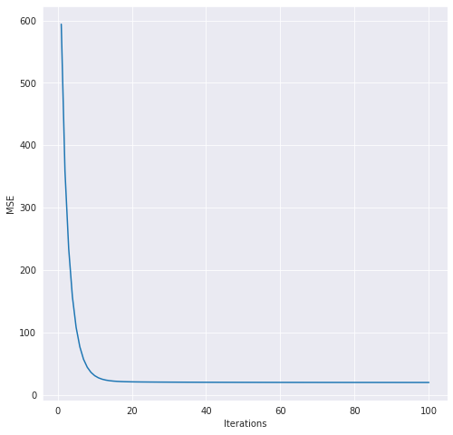
In order to demonstrate this implementation, I will use the prototypical Boston dataset. I will load the data, split it into train and test, use the standard scaler, and then perform the fitting. I will also output a lineplot so that you can see the progress of gradient descent in action.
import sklearn.datasets
from sklearn.preprocessing import StandardScaler
boston = sklearn.datasets.load_boston()
from sklearn.model_selection import train_test_split

# load the data
X = pd.DataFrame(boston.data, columns=boston.feature_names)
y = boston.target

# split the data
X_train, X_test, y_train, y_test = train_test_split(X,y, test_size = 0.3)

# scale the training data
scaler = StandardScaler()
X_train_scaled = scaler.fit_transform(X_train)
X_test_scaled = scaler.fit_transform(X_test)

# instantiate the model and fit to the scaled training data
lr = AndyLinRegGD(eta = 0.1, l2_reg = 0.01)
lr.fit(X_train_scaled, y_train, max_iter = 100)

# plot the gradient descent history
hist = lr.get_history()
plt.figure(figsize=(8,8))
sns.lineplot(x = 'Iterations', y = "MSE", data = hist)
<AxesSubplot:xlabel='Iterations', ylabel='MSE'>
Let’s also take a look at the history dataframe for gradient descent.
hist.head(5)
| Iterations | MSE | Updated Weights | |
|---|---|---|---|
| 0 | 1 | 593.982458 | [22.38926553220308, -0.870699471124182, 0.9237... |
| 1 | 2 | 358.076426 | [22.38926553220308, -0.870699471124182, 0.9237... |
| 2 | 3 | 234.355188 | [22.38926553220308, -0.870699471124182, 0.9237... |
| 3 | 4 | 157.144036 | [22.38926553220308, -0.870699471124182, 0.9237... |
| 4 | 5 | 108.103451 | [22.38926553220308, -0.870699471124182, 0.9237... |
hist.tail(5)
| Iterations | MSE | Updated Weights | |
|---|---|---|---|
| 95 | 96 | 19.646877 | [22.38926553220308, -0.870699471124182, 0.9237... |
| 96 | 97 | 19.645203 | [22.38926553220308, -0.870699471124182, 0.9237... |
| 97 | 98 | 19.643577 | [22.38926553220308, -0.870699471124182, 0.9237... |
| 98 | 99 | 19.641997 | [22.38926553220308, -0.870699471124182, 0.9237... |
| 99 | 100 | 19.640460 | [22.38926553220308, -0.870699471124182, 0.9237... |
Now that we have the model, let’s go ahead and create predictions for the test set and see how it performs
predictions = lr.predict(X_test_scaled)

mse = np.sum((predictions - y_test)**2)/len(y_test)

print("The MSE for the test set is", mse)
The MSE for the test set is 27.919555078006432
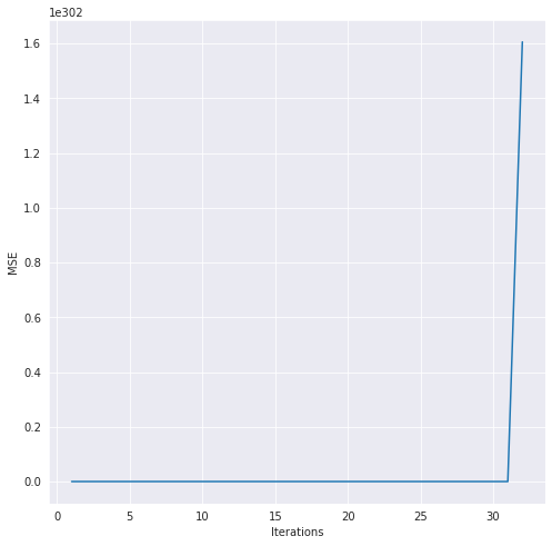
There it is! The model is at least functioning how I would expect. Before I end this post, I want to demonstrate how important scaling the data is before you fit the model to it. It took me so long to figure out why gradient descent wasn’t working, only to find out that scaling the data single-handedly fixed the issue. I never realized just how important it was, but for me, gradient descent just was not working at all. Here’s a demo so that you can see what I mean.
#Use the pre-scaled dataset and a new lr object
lr2 = AndyLinRegGD(eta = 0.1, l2_reg = 0.01)
lr2.fit(X_train, y_train)

# plot the gradient descent history, notice the scale on the y-axis
hist2 = lr2.get_history()
plt.figure(figsize=(8,8))
sns.lineplot(x = 'Iterations', y = "MSE", data = hist2)
/usr/local/lib/python3.6/site-packages/ipykernel_launcher.py:46: RuntimeWarning: overflow encountered in square
/usr/local/lib/python3.6/site-packages/ipykernel_launcher.py:29: RuntimeWarning: overflow encountered in multiply


<AxesSubplot:xlabel='Iterations', ylabel='MSE'>
hist2.head(10)
| Iterations | MSE | Updated Weights | |
|---|---|---|---|
| 0 | 1 | 1.178545e+05 | [nan, nan, nan, nan, nan, nan, nan, nan, nan, ... |
| 1 | 2 | 4.437804e+14 | [nan, nan, nan, nan, nan, nan, nan, nan, nan, ... |
| 2 | 3 | 1.707692e+24 | [nan, nan, nan, nan, nan, nan, nan, nan, nan, ... |
| 3 | 4 | 6.571943e+33 | [nan, nan, nan, nan, nan, nan, nan, nan, nan, ... |
| 4 | 5 | 2.529172e+43 | [nan, nan, nan, nan, nan, nan, nan, nan, nan, ... |
| 5 | 6 | 9.733367e+52 | [nan, nan, nan, nan, nan, nan, nan, nan, nan, ... |
| 6 | 7 | 3.745827e+62 | [nan, nan, nan, nan, nan, nan, nan, nan, nan, ... |
| 7 | 8 | 1.441559e+72 | [nan, nan, nan, nan, nan, nan, nan, nan, nan, ... |
| 8 | 9 | 5.547752e+81 | [nan, nan, nan, nan, nan, nan, nan, nan, nan, ... |
| 9 | 10 | 2.135019e+91 | [nan, nan, nan, nan, nan, nan, nan, nan, nan, ... |
hist2.tail(5)
| Iterations | MSE | Updated Weights | |
|---|---|---|---|
| 995 | 996 | NaN | [nan, nan, nan, nan, nan, nan, nan, nan, nan, ... |
| 996 | 997 | NaN | [nan, nan, nan, nan, nan, nan, nan, nan, nan, ... |
| 997 | 998 | NaN | [nan, nan, nan, nan, nan, nan, nan, nan, nan, ... |
| 998 | 999 | NaN | [nan, nan, nan, nan, nan, nan, nan, nan, nan, ... |
| 999 | 1000 | NaN | [nan, nan, nan, nan, nan, nan, nan, nan, nan, ... |
Isn’t that wild? I don’t really know what’s happening with the weights but you can see at least in the first ten iterations of gradient descent how the MSE just skyrockets instead of steadily decreasing. I can’t tell you much time I spent pouring over the gradient descent function in this project! Ultimately, now I know how important scaling can be to a linear regression model.
Thank you for taking the time to read through this post. If you notice any errors, inconsistencies, or opportunities to improve the code, please let me know! I want to eventually extend this to an elastic net/stochastic version, so any advice or tips would be very appreciated! Take care!